import pandas as pd
import numpy as np
import matplotlib.pyplot as plt
# Import the data
data = pd.read_csv("tracking.txt", sep='\t')
data
| xHead | yHead | tHead | xTail | yTail | tTail | xBody | yBody | tBody | |
|---|---|---|---|---|---|---|---|---|---|
| Float64 | Float64 | Float64 | Float64 | Float64 | Float64 | Float64 | Float64 | Float64 | |
| 1 | 514.327 | 333.12 | 5.81619 | 499.96 | 327.727 | 6.10226 | 508.345 | 330.876 | 5.94395 |
| 2 | 463.603 | 327.051 | 0.301279 | 449.585 | 330.323 | 0.245547 | 458.058 | 328.346 | 0.238877 |
| 3 | 23.9978 | 287.715 | 3.70646 | 34.9722 | 278.836 | 3.99819 | 29.2056 | 283.505 | 3.84844 |
| 4 | 372.536 | 230.143 | 0.194641 | 354.226 | 231.604 | 6.08737 | 364.822 | 230.759 | 0.0515087 |
| 5 | 480.58 | 213.482 | 1.28236 | 478.125 | 228.52 | 1.53303 | 479.428 | 220.543 | 1.42567 |
| 6 | 171.682 | 143.55 | 6.09077 | 155.507 | 140.116 | 6.1146 | 164.913 | 142.113 | 6.08216 |
| 7 | 498.151 | 121.32 | 6.00177 | 483.712 | 119.285 | 0.0223247 | 492.683 | 120.55 | 6.15298 |
| 8 | 329.56 | 123.418 | 6.08726 | 312.526 | 119.042 | 5.9098 | 322.531 | 121.614 | 6.01722 |
| 9 | 465.256 | 115.045 | 4.44359 | 470.057 | 99.911 | 4.40559 | 467.106 | 109.205 | 4.40862 |
| 10 | 423.663 | 66.3789 | 0.0888056 | 409.105 | 67.2971 | 6.12053 | 417.615 | 66.7623 | 0.0292602 |
| 11 | 424.487 | 40.4232 | 5.48198 | 411.594 | 30.3912 | 5.88869 | 418.96 | 36.1192 | 5.64923 |
| 12 | 370.591 | 35.2147 | 5.99688 | 354.672 | 29.5633 | 5.89121 | 364.007 | 32.8767 | 5.94008 |
| 13 | 498.502 | 20.2527 | 5.66339 | 487.254 | 9.19499 | 5.39497 | 493.758 | 15.5781 | 5.5026 |
| 14 | 367.791 | 5.03034 | 6.05933 | 352.076 | 6.75603 | 0.653641 | 361.12 | 5.75904 | 0.152688 |
| 15 | 512.965 | 332.575 | 5.86617 | 499.435 | 327.759 | 6.052 | 507.626 | 330.673 | 5.95102 |
| 16 | 463.385 | 324.659 | 0.707 | 451.431 | 332.193 | 0.246265 | 458.959 | 327.443 | 0.542368 |
| 17 | 19.4579 | 293.022 | 4.28861 | 25.5579 | 281.206 | 4.18379 | 21.8962 | 288.302 | 4.23379 |
| 18 | 379.037 | 230.527 | 6.10571 | 361.728 | 229.616 | 0.199343 | 371.74 | 230.144 | 6.25939 |
| 19 | 478.884 | 206.712 | 1.27832 | 475.454 | 221.757 | 1.40929 | 477.197 | 214.108 | 1.35472 |
| 20 | 173.923 | 143.042 | 0.00732468 | 157.261 | 142.182 | 6.00453 | 167.066 | 142.689 | 6.20403 |
| 21 | 498.561 | 122.687 | 5.83253 | 486.357 | 118.196 | 6.13893 | 493.718 | 120.906 | 5.95151 |
| 22 | 328.812 | 124.134 | 6.05932 | 312.848 | 119.605 | 5.98617 | 322.331 | 122.294 | 6.00901 |
| 23 | 461.738 | 116.731 | 4.47649 | 466.371 | 101.736 | 4.40285 | 463.615 | 110.656 | 4.41641 |
| 24 | 428.631 | 69.2715 | 5.87139 | 415.665 | 64.6444 | 6.13862 | 423.218 | 67.3364 | 5.96558 |
| 25 | 425.821 | 44.9942 | 5.59983 | 414.84 | 33.2028 | 5.37159 | 421.248 | 40.0897 | 5.461 |
| 26 | 368.362 | 35.6219 | 5.97427 | 353.22 | 30.4625 | 5.88261 | 362.109 | 33.4891 | 5.94605 |
| 27 | 503.484 | 22.7293 | 5.76026 | 489.632 | 16.6315 | 5.92136 | 497.924 | 20.2857 | 5.86668 |
| 28 | 369.184 | 5.84074 | 6.15994 | 352.622 | 4.25328 | 6.24787 | 362.144 | 5.16766 | 6.19236 |
| 29 | 510.519 | 331.417 | 5.88883 | 495.784 | 327.366 | 6.12889 | 504.484 | 329.758 | 6.02088 |
| 30 | 464.242 | 323.533 | 0.290639 | 451.756 | 328.194 | 0.532686 | 459.432 | 325.326 | 0.37736 |
| ⋮ | ⋮ | ⋮ | ⋮ | ⋮ | ⋮ | ⋮ | ⋮ | ⋮ | ⋮ |
# Count the number of detected object
objectNumber = len(set(data["id"].values))
objectNumber
2
# Count the number of image
imageNumber = np.max(data["imageNumber"]) + 1
imageNumber
2000
# Plot the number of objects detected by frame
objectByFrame = np.zeros(imageNumber)
for i in range(imageNumber):
    objectByFrame[i] = data[data["imageNumber"] == i].shape[0]

plt.scatter(range(imageNumber), objectByFrame)
<matplotlib.collections.PathCollection at 0x7fa41831c6d8>

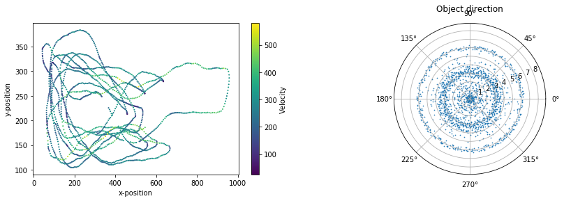
# Plot the trajectory of the first object and its orientation
dataObject0 = data[data["id"] == 0]
distance = np.sqrt(np.diff(dataObject0["xBody"].values)**2 + np.diff(dataObject0["yBody"].values)**2)
framerate = 50
time = np.diff(dataObject0["imageNumber"].values)/framerate
velocity = distance/time

fig, ax = plt.subplots(1, 2)
fig.subplots_adjust(right = 2)

ax[0] = plt.subplot(121)
plot = ax[0].scatter(dataObject0["xBody"][0:-1], dataObject0["yBody"][0:-1], c = velocity, s = 1)
ax[0].set_xlabel("x-position")
ax[0].set_ylabel("y-position")
bar = fig.colorbar(plot)
bar.set_label("Velocity")

ax[1] = plt.subplot(122, projection='polar')
ax[1].scatter(range(dataObject0["tBody"].shape[0]), dataObject0["tBody"], s = 0.4)
ax[1].set_title("Object direction")
Text(0.5, 1.05, 'Object direction')